Doing less work: the algorithm behind uv's 12,000x benchmark

An exploration of Boolean logic, decision diagrams, and the surprising difference between doing less work and doing work faster.

Imagine that I give you a rather peculiar job.

I have a large collection of switches. Each switch can be either on or off. Depending on which switches are on, a machine will either run or refuse to run.

Your task is to write down the rules governing this machine.

You might say, “Well, that’s easy enough. I’ll try every possible combination of switches, see which ones make the machine run, and write those combinations down.”

Perfectly reasonable.

And, as we’re about to discover, potentially disastrous.

That tension between a compact rule and a long list of cases will help us understand a problem that Charlie Marsh and the developers of uv encountered. uv is a Python package and project manager written in Rust. Its software needed to translate logical conditions from one representation into another. The existing approach worked well for small problems, but on certain complicated inputs, it became extraordinarily slow.

In his October 20 post on X, Marsh credits Astra with finding and implementing the Minato-Morreale Irredundant Sum of Products (ISOP) recurrence.

In the pull request’s reported comparison, one internal marker-formatting benchmark went from taking approximately 1.31 seconds to just 0.11 milliseconds.

That’s nearly 12,000 times faster.

Now, the interesting question isn’t really how fast it became.

The interesting question is: What was the computer doing that was so unnecessary in the first place?

To understand that, we need to begin with something almost embarrassingly simple.

You can follow the explanation from the beginning, then try the ten problems before reading the worked solutions.

---

1. A Machine With Three Switches

Suppose we have three switches, A, B, and C.

The machine runs under either of these conditions:

• A and B are both on.
• A is off, but C is on.

In mathematical notation, we write:

$$F=(A\land B)\lor(\neg A\land C)$$

The symbol $\land$ means AND, $\lor$ means OR, and $\neg$ means NOT.

Nothing mysterious.

Let’s try some combinations.

If A is on and B is on, the machine runs. We don’t care about C.

If A is off and C is on, the machine runs. We don’t care about B.

Already, we’ve discovered something important: not every switch matters in every situation.

But suppose we don’t know these simple rules. Suppose all we have is a table showing what happens for every combination.

A	B	C	Machine runs?
0	0	0	No
0	0	1	Yes
0	1	0	No
0	1	1	Yes
1	0	0	No
1	0	1	No
1	1	0	Yes
1	1	1	Yes

We could write a separate rule for every row where the machine runs.

For instance, the second row says:

$$\neg A\land\neg B\land C$$

The fourth row says:

$$\neg A\land B\land C$$

And so on.

Combining all four successful combinations gives:

$$\begin{aligned} F={}&(\neg A\land\neg B\land C)\\ &\lor(\neg A\land B\land C)\\ &\lor(A\land B\land\neg C)\\ &\lor(A\land B\land C) \end{aligned}$$

This expression is completely correct.

But it’s terribly wasteful.

Look at the first two terms. They both require A to be off and C to be on. The only difference is B.

One term says B must be off. The other says B must be on.

But B must be one or the other!

So B doesn’t matter at all.

We can replace those two terms with:

$$\neg A\land C$$

Likewise, the final two terms collapse into:

$$A\land B$$

And we’re back to:

$$\boxed{F=(A\land B)\lor(\neg A\land C)}$$

Four complicated rules have become two simple ones.

What we’ve done is called Boolean simplification.

And the long expression we started with is an example of Disjunctive Normal Form, or DNF.

---

2. What Exactly Is DNF?

Despite its imposing name, Disjunctive Normal Form is simply a particular way of writing logical expressions.

A DNF expression consists of groups of conditions connected by AND, with those groups connected by OR.

For example:

$$(A\land B)\lor(C\land\neg D)\lor E$$

Each AND-connected group is called a product term, or sometimes a cube.

The OR connecting these terms is called a sum.

That’s why mathematicians also call DNF a Sum of Products.

Here, “sum” means OR and “product” means AND. These are Boolean operations, rather than ordinary addition and multiplication.

You might wonder why we bother with such a rigid format.

The answer is that a standardized representation is convenient for computers. If every logical expression is written in the same general form, we can systematically compare, combine, and manipulate expressions.

This common format does not make DNF unique. Our four-term and two-term expressions describe the same function, even though they look different. Checking equivalence still takes reasoning.

And every Boolean function of finitely many Boolean inputs can be expressed in DNF.

That’s an extremely useful property.

Unfortunately, it comes with a rather nasty complication.

The trouble with counting combinations

Our three-switch machine has:

$$2^3=8$$

possible switch combinations.

If we have ten switches:

$$2^{10}=1024$$

If we have thirty:

$$2^{30}=1{,}073{,}741{,}824$$

That’s over a billion combinations.

Now imagine that the machine runs whenever switch A is on, regardless of the other twenty-nine switches.

The complete rule is simply:

$$F=A$$

One letter.

But if we blindly enumerate every successful combination, we’ll generate:

$$2^{29}=536{,}870{,}912$$

different terms.

More than half a billion terms to express something that could have been written with one letter.

And then, after generating those half-billion terms, we might attempt to simplify them back into A.

Can you see the absurdity?

We’ve created an enormous problem for ourselves, only to spend even more effort undoing it.

The computer isn’t slow because the answer is complicated. It’s slow because the procedure for finding the answer is complicated.

Suppose I ask you whether this machine will run. You already know its rule is $F=A$. What do you look at?

A. That’s all.

If A is on, answer yes. If A is off, answer no. You don’t even look at the other twenty-nine switches.

Draw that on a piece of paper: one question about A, with a yes branch and a no branch. You have just made a decision diagram.

uv had already taken this step. It stored conditions as diagrams. Its trouble came when it needed to turn those diagrams back into written rules.

Let’s draw one for our three-switch machine and see how that works.

---

3. A Better Way to Think About Switches

Instead of writing down every combination, suppose we construct a little decision-making machine.

It asks questions.

First: Is A on?

If A is on, ask whether B is on. If B is also on, the machine runs.

If A is off, ask whether C is on. If C is on, the machine runs.

We can draw this as a graph:

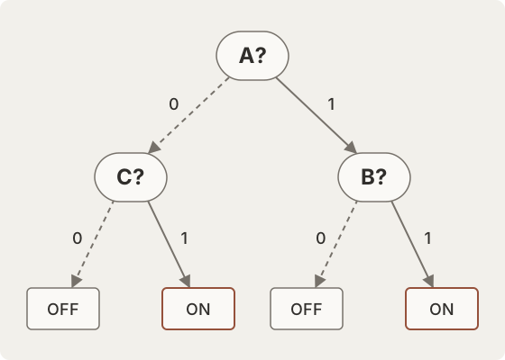
A dashed branch means the switch is off (0); a solid branch means it is on (1). Try A off and C on: take the 0 branch from A, then the 1 branch from C. You reach ON without ever asking about B.

This is the basic idea behind a Binary Decision Diagram (BDD).

A BDD represents a Boolean function as a network of decisions.

Each internal node tests a variable. Each branch represents the result of that test. Eventually, we reach TRUE or FALSE.

A particularly useful variant, the Reduced Ordered Binary Decision Diagram (ROBDD), keeps variables in a fixed order along each path, eliminates unnecessary tests, and shares identical subgraphs.

That sharing is important.

Suppose two different paths eventually lead to exactly the same decision. Instead of storing two copies of that decision, we can store one and let both paths point to it.

It’s rather like writing a computer program with reusable functions instead of copying the same code everywhere.

For many Boolean functions, the resulting graph is dramatically smaller than the corresponding truth table.

But now we encounter an unexpected problem.

The graph isn’t the final answer

A Python package manager such as uv needs to work with conditions like:

python_version >= "3.11"

or:

sys_platform == "win32"

These are called environment markers.

They tell the package manager when particular dependencies apply. The Python packaging specification defines how these marker expressions are interpreted, including their version comparisons.

Internally, uv can represent complicated combinations of these conditions using decision diagrams. As Marsh explains in his thread, this helps it combine conditions and check whether they are equivalent or satisfiable.

Its actual diagrams also handle version and string ranges. Our switches isolate the Boolean part so we can understand the idea before returning to those extra details.

But when uv writes a lockfile, it needs to turn those diagrams back into expressions.

In other words, it needs to go from a graph to a logical formula.

And this is where things get interesting.

---

4. The Tempting but Expensive Solution

Suppose you’re given a decision diagram and asked to produce its DNF.

There’s a straightforward method.

Start at the top of the graph. Follow every possible path that ends at TRUE. For each successful path, write down the conditions encountered along the way.

Then connect all those path expressions with OR.

You’ve produced a DNF.

Congratulations!

Except there’s a problem.

A decision diagram can be compact precisely because it shares subgraphs. When you enumerate all paths, you may undo that compactness.

A graph with a manageable number of nodes can contain an enormous number of paths.

And if you generate an expression for every successful path, you can end up with a gigantic DNF.

You then have to compare terms, discover redundancies, and simplify the whole thing.

What sharing saves, and path enumeration loses

Consider a different rule:

$$F = (A \land B) \lor (C \land D)$$

Test A, then B if necessary. If the first pair fails, test C and D. Both ways of failing the first pair can point to the same C node:

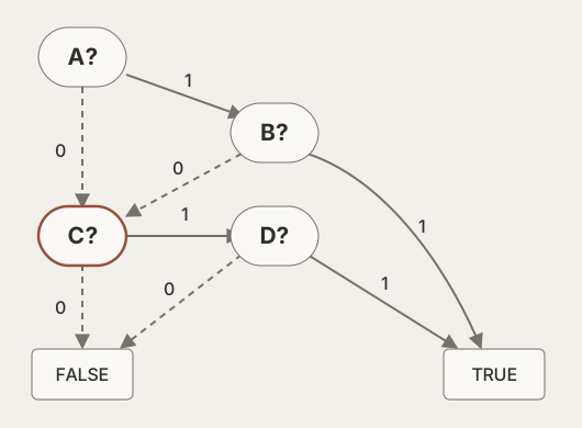
Dashed branches mean false (0); solid branches mean true (1). C and D are shared decisions.

There are four internal decision nodes. But collecting every path to TRUE produces three terms:

$$\begin{aligned} & (A \land B) \\ &\lor (\neg A \land C \land D) \\ &\lor (A \land \neg B \land C \land D) \end{aligned}$$

These paths are mutually exclusive: each records a different route through the graph. The shorter expression allows overlap. When all four switches are on, both $A \land B$ and $C \land D$ hold, and that is perfectly fine.

That freedom matters. We want an expression describing when the machine runs; we do not need to preserve the route taken through the graph.

Now extend the pattern:

$$(A_1 \land B_1) \lor (A_2 \land B_2) \lor \cdots \lor (A_n \land B_n)$$

With the variables ordered by pairs, this BDD needs $2n$ internal nodes. Each failed pair has two possible routes: A is false, or A is true and B is false. The number of paths to TRUE is therefore:

$$1 + 2 + 4 + \cdots + 2^{n-1} = 2^n - 1$$

At 20 pairs, that is 40 decision nodes and 1,048,575 successful paths, even though the rule already has a DNF with only 20 terms.

This is a constructed example of how path enumeration can grow. It is not one of uv’s benchmark fixtures.

Back to uv

This was the broad approach used in uv before the optimization. Its old conversion code collected paths to TRUE, simplified the resulting DNF, and sorted the clauses. Marsh describes the same sequence in his explanation.

It worked well for small expressions.

But certain complicated dependency resolutions produced enormous intermediate expressions, and simplifying them became extremely expensive.

The computer was spending a tremendous amount of time generating unnecessary terms and then removing them.

So we should ask a different question.

Why generate those unnecessary terms at all?

---

5. The Mathematical Trick: Split the Problem in Two

There’s a beautiful identity in Boolean algebra called the Shannon expansion.

For any Boolean function $F$, choose a variable $x$.

We can always write:

$$\boxed{F=(\neg x\land F_0)\lor(x\land F_1)}$$

Here:

• $F_0$ is what remains of F when x is false.
• $F_1$ is what remains of F when x is true.

These smaller functions are called cofactors. We have fixed one switch and asked what rule remains for the others.

Let’s try it with:

$$F=A\lor B$$

Choose A as our variable.

If A is false, the function becomes B.

If A is true, the function becomes TRUE, regardless of B.

Therefore:

$$F=(\neg A\land B)\lor(A\land 1)$$

Since $A\land1=A$:

$$F=(\neg A\land B)\lor A$$

Now comes a clever observation.

If A is true, the expression is already true.

If A is false, B determines the answer.

Therefore, the whole thing can be written:

$$\boxed{F=A\lor B}$$

The Shannon expansion allows us to break a complicated function into smaller functions.

And smaller functions can be broken down again.

And again.

This is the foundation of many recursive algorithms for Boolean logic.

But there’s another opportunity hiding here.

Notice that sometimes the two branches can be combined into a term that doesn’t mention the variable we’re splitting on.

For example:

$$(\neg A\land B)\lor(A\land B)=B$$

Both branches require B.

So A is irrelevant.

What if our algorithm could recognize such opportunities while constructing the answer, instead of discovering them only after producing a giant expression?

That brings us to Minato and Morreale.

---

6. The Minato-Morreale ISOP Recurrence

ISOP stands for Irredundant Sum of Products.

Let’s unpack that.

We already know that Sum of Products is another name for DNF.

What does irredundant mean?

Suppose our expression is:

$$F=A\lor(A\land B)$$

The second term contributes nothing.

Whenever $A\land B$ is true, A is already true.

So we can remove the second term:

$$F=A$$

The original expression was redundant. The simplified expression is irredundant.

A cover is a collection of product terms whose OR covers the required cases. For an exact function, a cover is term-irredundant when no complete product term can be removed without changing that function.

There is a second kind of unnecessary detail: a condition inside a term. If dropping a literal, such as A or its negation, would make a term include a case outside the function, that literal is necessary. A term is prime when none of its literals can be dropped without doing that.

Notice the difference. In $(\neg A\land B)\lor(A\land B)$, neither whole term can simply be deleted. Yet the condition on A can be removed, and the expression can become B. Checking only for removable terms would miss this simplification.

For Boolean functions, the ISOP construction gives a prime, term-irredundant cover. Some authors use “irredundant” for that combination of properties, as in Minato and De Micheli’s definition.

Notice that irredundant doesn’t necessarily mean globally smallest. There may be several irredundant representations of the same function, some larger than others.

Now, the Minato-Morreale recurrence is a recursive method for constructing such a cover directly from a Boolean function represented by a decision diagram.

The crucial innovation is that it doesn’t simply enumerate every successful path.

It reasons about what each branch must cover, and what can be covered without distinguishing between the branches.

The three-part decomposition

Imagine splitting a function on variable x.

The resulting expression can be organized into three parts:

$$\boxed{P=(\neg x\land P_0)\lor(x\land P_1)\lor P_2}$$

The first part handles conditions that specifically need x to be false.

The second handles conditions that specifically need x to be true.

And the third handles conditions that don’t need to mention x at all.

That third part is the particularly interesting one.

Consider:

$$F=(\neg A\land B)\lor(A\land B)$$

A naive approach might preserve two separate branches.

But both branches are covered by B.

So the third part can simply be:

$$P_2=B$$

And the entire expression becomes B.

We’ve eliminated the distinction between A being true and false.

A reduced BDD for this particular function would already have omitted A. Here, the algebra lets us see why omitting a variable is valid. Next, we need to understand how the recurrence finds such opportunities as it builds a cover.

This is how we avoid constructing many unnecessary terms.

Where don’t-care conditions enter

The full algorithm is a little more sophisticated than that example suggests.

It works with a lower bound $L$ and an upper bound $U$, satisfying:

$$L\Rightarrow U$$

We want to construct an expression $P$ such that:

$$L\Rightarrow P\Rightarrow U$$

Think of L as the cases we absolutely must include, and U as the cases we’re allowed to include.

Anything outside U must be excluded.

But in the region where U is true and L is false, the algorithm has freedom.

These are called don’t-care conditions.

Why are don’t-cares useful?

Suppose you’re designing a circuit and certain input combinations can never occur. You don’t need to preserve a particular output for those impossible combinations.

You can choose whichever output makes the circuit simpler.

The ISOP recurrence exploits similar freedom in its recursive subproblems.

By carefully choosing what each branch needs to cover, it can avoid introducing terms that later turn out to be unnecessary.

When we initially want an exact representation of F, we start with:

$$L=U=F$$

The recursive algorithm then constructs smaller constrained problems where useful don’t-care regions arise. Other parts of the cover can handle some cases, so a particular recursive call has freedom in how it handles them.

At the top level, every original input still has a fixed answer. We are distributing responsibility among parts of the cover, not changing when the original machine runs.

The mathematical details are intricate, but the organizing principle is remarkably simple:

Cover what must be covered, exclude what must be excluded, and use the remaining freedom to simplify the result.

Follow one small ISOP calculation

Let’s use $F=A\lor B$ again and split on A. If A is false, both bounds become B. If A is true, both bounds become 1, where 1 means TRUE.

The Boolean recurrence, described in section 4.1, constructs the three pieces in order. For this example, its subproblems look like this:

Part	Cases it must cover	Cases it may cover	Chosen cover
$P_0$	$0$	$B$	$0$
$P_1$	$\neg B$	$1$	$1$
$P_2$	$B$	$B$	$B$

The false-A part has nothing it must cover, so $P_0=0$ works.

The true-A part must cover B being false, but it is allowed to cover B being true too. The constant 1 is therefore a valid answer for this recursive subproblem. Put A back in front of it, and that contribution is simply A.

The remaining common part is B. It can omit A, because B is permitted in both branches.

Now assemble the pieces:

$$\begin{aligned} P &= (\neg A\land 0)\lor(A\land 1)\lor B \\ &= A\lor B \end{aligned}$$

When A and B are both true, the two final terms overlap. That causes no problem. OR only asks whether at least one term holds; it does not require each successful case to belong to exactly one term.

What uv actually implements

There is one boundary to keep in mind as we return to the package manager. uv’s Rust implementation uses the Minato-Morreale recurrence for Boolean decisions and adapts cover extraction to version and string ranges.

The code explicitly says that the range-based extension preserves the function but does not guarantee a prime, irredundant cover over arbitrary unions of ranges. So our Boolean discussion explains the central idea; it does not establish that every marker expression uv emits is irredundant or globally smallest.

---

7. Why Remembering Previous Work Matters

There’s one more important ingredient: memoization.

Suppose you’re solving a complicated problem recursively.

You split it into two smaller problems.

Each of those splits into more problems.

Eventually, you may encounter exactly the same subproblem several times.

A naive recursive algorithm solves it again every time.

A memoized algorithm remembers the answer.

If it encounters the same subproblem again, it retrieves the stored result.

Now consider a decision diagram.

Because different paths can share subgraphs, repeated subproblems arise naturally.

The Minato-Morreale algorithm can exploit this by caching results for previously encountered recursive states.

Instead of recomputing an equivalent cover for the same pair of Boolean bounds, it reuses the result.

This doesn’t guarantee polynomial-time performance. Boolean minimization remains computationally difficult in general, and some functions require exponentially large DNFs even when their decision diagrams are small. A large final answer still takes work to write down. Memoization helps avoid repeated work; it cannot make the output cost disappear.

But on many practical inputs, avoiding repeated computation and unnecessary intermediate terms makes an enormous difference.

And in uv’s case, it made a spectacular difference.

---

8. From 1.31 Seconds to 0.11 Milliseconds

Let’s return to Charlie Marsh’s pull request.

The pull request’s benchmark comparison included the following. All timings are in microseconds ($\mu\mathrm{s}$); lower is better:

Operation	Before ($\mu\mathrm{s}$)	After ($\mu\mathrm{s}$)	Reported speedup
Two-clause DNF	0.670	0.433	$1.5\times$
Sparse DNF, 512 clauses	13,239.5	65.0	$204\times$
Conflict DNF, 32 extras	483,748.7	46.0	$10{,}500\times$
Conflict-dependent formatting, 32 extras	1,312,396.2	109.9	$11{,}900\times$

The final row is about 1.31 seconds versus 0.11 milliseconds. The displayed timings yield roughly $11{,}942\times$, the table reports a rounded $11{,}900\times$ (and the X post rounds the headline to about $12{,}000\times$).

The simplest cases improved modestly.

The difficult cases improved enormously.

That pattern tells us something.

The old approach could generate huge intermediate DNFs and then spend time simplifying them.

The new approach constructs a simplified cover directly, avoiding much of that intermediate expansion. The Boolean recurrence and the range-handling qualification we discussed above explain what is, and is not, guaranteed about that cover.

We should be careful about interpreting the headline, however.

The benchmark does not mean that every uv command, or every Python installation, is now 12,000 times faster.

It means that a particular internal operation became nearly 12,000 times faster on one especially challenging test case.

Still, that’s an extraordinary result.

---

9. What Did the AI Actually Discover?

Here’s an important distinction.

The AI did not invent the Minato-Morreale recurrence.

The underlying mathematical research already existed. Minato and De Micheli’s paper describes the Minato-Morreale algorithm and cites earlier work by Minato and Morreale.

As Marsh describes it, the achievement was identifying that this algorithm could be applied to uv’s particular problem and implementing the change. That is his account of the development process; the public benchmark measures the resulting code.

That’s an interesting form of problem-solving.

Imagine you’re working on a package manager. You might naturally look for ways to optimize dependency resolution, improve caching, or speed up individual marker operations.

But the bottleneck turns out to be closely related to a problem studied in logic synthesis and Boolean function minimization.

The solution comes not from package management itself, but from another area of computer science.

That kind of connection is extremely valuable.

And it’s one of the more promising uses of AI coding agents: helping developers find and apply techniques from areas they might not have considered.

Of course, identifying an algorithm is only part of the work. Correct implementation, equivalence testing, performance measurement, and handling edge cases remain essential.

A faster algorithm that produces the wrong dependency conditions would be a very serious regression.

---

10. The Deeper Lesson: Sometimes the Best Calculation Is the One You Never Perform

Let’s revisit our thirty-switch machine.

We wanted to determine when the machine runs.

The answer was simply:

$$F=A$$

One possible approach would be to enumerate over half a billion successful switch combinations, write them down, and then simplify the result.

Another approach would be to reason about the structure of the problem and discover that the other twenty-nine switches don’t matter.

Both approaches can lead to the same answer.

But one of them performs an extraordinary amount of unnecessary work.

This is a recurring theme throughout computer science.

A good algorithm isn’t merely a faster way to perform the same sequence of operations.

Sometimes it changes the sequence entirely.

Sometimes it changes how the problem is represented.

And sometimes it discovers that most of the work we thought was necessary wasn’t necessary at all.

The Minato-Morreale recurrence is a beautiful example of this idea.

Instead of producing an enormous logical expression and struggling to simplify it, the algorithm uses the structure of the Boolean function to construct a much cleaner expression from the beginning.

And perhaps the most delightful part of the story is that an algorithm from Boolean logic research found a practical application inside a modern Python package manager, with an AI coding agent helping make the connection.

---

11. Now It’s Your Turn: Problems Worth Thinking About

Reading an explanation and understanding it are two different things.

There’s a simple way to find out whether we’ve really understood something: try to use it.

The following problems begin with elementary Boolean logic and gradually approach the ideas behind the Minato-Morreale recurrence.

Don’t worry about memorizing formulas. Try to reason about what each expression actually says.

Difficulty guide: Beginner, Intermediate, Advanced.

Problem 1: The Security System (Beginner)

A security system has three sensors:

• A detects an open door.
• B detects a broken window.
• C detects movement.

The alarm activates if both the door and window sensors trigger, or if the motion sensor triggers regardless of the other sensors.

Questions:

1. Write the alarm condition in DNF.
2. How many possible sensor combinations exist?
3. How many combinations activate the alarm?
4. Is the expression already irredundant?

Problem 2: Four Rules, or Just One? (Beginner)

Consider:

$$\begin{aligned} F={}&(A\land B\land C)\\ &\lor(A\land B\land\neg C)\\ &\lor(A\land\neg B\land C)\\ &\lor(A\land\neg B\land\neg C) \end{aligned}$$

Questions:

1. Simplify the expression as far as possible.
2. Which variables actually affect the result?
3. Explain why the original expression is unnecessarily complicated.

Problem 3: The Growing Truth Table (Intermediate)

A system has 16 Boolean inputs, including A. Its output is TRUE exactly when A is TRUE; the other 15 inputs do not affect the output.

Questions:

1. How many possible assignments are there?
2. How many assignments satisfy the function?
3. How many terms would its canonical truth-table DNF contain?
4. How many terms does its simplest DNF contain?
5. What happens to these counts if the number of inputs doubles to 32?

Problem 4: Build a Decision Diagram (Intermediate)

Consider:

$$F=(A\land B)\lor(\neg A\land C)$$

Construct a decision diagram with A as the first variable tested.

Questions:

1. Which variable should be tested when A is FALSE?
2. Which variable should be tested when A is TRUE?
3. How many distinct internal decision nodes are needed?
4. Write the two cofactors $F_0$ and $F_1$ with respect to A.
5. Verify that Shannon expansion reconstructs the original expression.

Problem 5: Find the Unnecessary Term (Intermediate)

Consider:

$$F=A\lor(A\land B)\lor(B\land C)$$

Questions:

1. Which product term can be removed?
2. Write the resulting irredundant DNF.
3. Explain why removing that term doesn’t change the function.
4. Can either of the remaining terms be removed?

Problem 6: The Variable That Disappeared (Advanced)

Consider:

$$F=(\neg A\land B)\lor(A\land B)\lor(A\land C)$$

Questions:

1. Simplify the first two terms.
2. Write the resulting DNF.
3. Which part of the result no longer depends on A?
4. Relate this to the $P_2$ component in the three-part ISOP decomposition.

Problem 7: Understanding Don’t-Care Conditions (Advanced)

Suppose a system has two Boolean inputs A and B.

Its output requirements are:

A	B	Required output
0	0	0
0	1	Don’t care
1	0	1
1	1	1

Questions:

1. What is the simplest expression satisfying these requirements?
2. What happens if the don’t-care output is chosen as TRUE?
3. What happens if it is chosen as FALSE?
4. Why can don’t-care conditions help simplify Boolean expressions?

Problem 8: Thinking Like an Algorithm Designer (Advanced)

You are implementing a function that converts a decision diagram into DNF.

You have two possible approaches:

Algorithm A: Enumerate every path leading to TRUE, construct a DNF, and simplify it afterward.

Algorithm B: Recursively construct an irredundant cover, exploiting shared subproblems and don’t-care conditions.

Questions:

1. Which algorithm is more likely to perform unnecessary work on highly repetitive Boolean functions?
2. Why might Algorithm B be substantially faster?
3. Does Algorithm B guarantee polynomial-time performance for every Boolean function?
4. Why is memoization especially useful when working with decision diagrams?
5. Return to the OR-of-pairs example in section 4. For ten pairs, how many internal decision nodes, paths to TRUE, and terms in the compact DNF are there?

Problem 9: A Small ISOP Challenge (Advanced)

Let the lower and upper bounds be:

$$L=A\land B$$ $$U=A\lor B$$

We want an expression $P$ satisfying:

$$L\Rightarrow P\Rightarrow U$$

Questions:

1. Is $P=A$ valid?
2. Is $P=B$ valid?
3. Is $P=A\lor B$ valid?
4. Is $P=1$ valid?
5. Why can several different expressions satisfy the same lower and upper bounds?

Problem 10: The Engineering Judgment (Advanced)

A benchmark shows that a new algorithm runs 11,900 times faster on a difficult input, but only 1.5 times faster on a simple input.

Questions:

1. Does this prove the entire application is 11,900 times faster?
2. What might explain the much larger speedup on complicated inputs?
3. What correctness tests would you perform before accepting the optimization?
4. How would you investigate whether the new algorithm improves real-world performance?

---

12. Answer Key and Explanations

Try the problems before reading this section. The goal is not merely to obtain the right answer, but to understand why it is right.

Solution 1

The alarm condition is:

$$F=(A\land B)\lor C$$

There are $2^3=8$ possible sensor combinations.

Four combinations have C TRUE. Of the four combinations where C is FALSE, only one has both A and B TRUE.

Therefore, five combinations activate the alarm.

The expression is irredundant because neither term can be removed without changing the result.

Solution 2

Factor out A:

$$F=A\land[(B\land C)\lor(B\land\neg C)\lor(\neg B\land C)\lor(\neg B\land\neg C)]$$

The expression inside the brackets covers every possible combination of B and C.

It is therefore always TRUE.

So:

$$\boxed{F=A}$$

Only A affects the result.

Solution 3

For 16 inputs:

$$2^{16}=65{,}536$$

Half the assignments satisfy A:

$$2^{15}=32{,}768$$

The canonical DNF contains 32,768 terms, but the simplest DNF contains just one: A.

For 32 inputs, the total number of assignments is:

$$2^{32}=4{,}294{,}967{,}296$$

The number of satisfying assignments, and therefore the number of canonical truth-table DNF terms, is:

$$2^{31}=2{,}147{,}483{,}648$$

The simplest DNF still has one term, A. Increasing the number of irrelevant inputs changes the truth-table size, but it does not change the rule.

Solution 4

When A is FALSE, test C.

When A is TRUE, test B.

The two cofactors are:

$$F_0=C,\qquad F_1=B$$

Shannon expansion gives:

$$F=(\neg A\land C)\lor(A\land B)$$

Three distinct internal decision nodes are sufficient: A, B, and C.

Solution 5

The redundant term is:

$$A\land B$$

Because whenever $A\land B$ is TRUE, A is already TRUE.

Therefore:

$$\boxed{F=A\lor(B\land C)}$$

Neither remaining term can be removed. For example, A covers the assignment $A=1,B=0,C=0$, while $B\land C$ covers $A=0,B=1,C=1$.

Solution 6

The first two terms combine:

$$(\neg A\land B)\lor(A\land B)=B$$

Therefore:

$$\boxed{F=B\lor(A\land C)}$$

The term B no longer depends on A. The whole function still can: if B is false and C is true, changing A changes the output. It is a condition inside one part of the expression that disappeared.

This illustrates the intuition behind the $P_2$ component: covering assignments with a term that doesn’t need to distinguish between the two values of the selected variable.

Solution 7

The simplest expression is:

$$\boxed{F=A}$$

Choosing FALSE for the don’t-care row produces exactly A.

Choosing TRUE instead produces $A\lor B$, which is also valid but requires an additional literal.

Don’t-care conditions provide freedom to choose whichever valid behavior makes the representation simpler.

Solution 8

Algorithm A is more likely to generate unnecessary intermediate expressions.

Algorithm B can avoid constructing redundant terms and reuse results for repeated subproblems.

However, Algorithm B does not guarantee polynomial-time performance for every Boolean function.

Memoization is useful because decision diagrams often contain shared subgraphs, so recursive computations can encounter identical subproblems.

For ten pairs, there are $2n=20$ internal decision nodes and $2^n-1=1023$ paths to TRUE. The compact DNF has ten terms. A path records the route taken through the graph; a term only needs to describe a sufficient condition for the output to be true.

Solution 9

We need:

$$A\land B\Rightarrow P\Rightarrow A\lor B$$

Both $P=A$ and $P=B$ are valid.

$P=A\lor B$ is also valid, as is $P=A\land B$.

But $P=1$ is invalid because it would be TRUE when both A and B are FALSE, violating the upper bound.

Multiple solutions exist because the bounds leave some assignments unconstrained. These examples satisfy the bounds; that does not mean the ISOP recurrence will return every one of them, or that each is equally economical for covering the required cases.

Solution 10

No, a speedup in one internal operation doesn’t imply the entire application improves by the same factor.

The larger speedup on difficult inputs suggests the new algorithm avoids work that grows rapidly under the old approach.

Correctness testing should include exhaustive equivalence checks for small functions, randomized tests for larger functions, edge cases, and regression tests against the previous implementation.

Performance testing should measure representative real-world workloads, not just synthetic worst cases.

---

A Final Question

Suppose you encounter an algorithm that’s running slowly.

Your first instinct might be to optimize its loops, reduce memory allocations, parallelize the computation, or move it to faster hardware.

Those are all reasonable possibilities.

But before doing any of them, ask yourself:

Is the computer doing work that doesn’t need to be done at all?

That question may be worth more than a thousand micro-optimizations.

---

Further exploration: Boolean algebra, Shannon expansion, Reduced Ordered Binary Decision Diagrams (ROBDDs), logic minimization, and Shin-ichi Minato’s work on irredundant sum-of-products generation.